GIS5100 Module 6 - Rapid Damage Assessment

Understanding the big picture of Damage Assessment 

Damage Assessment (DA) is a broad term that consists of multiple components and is itself a member of a much larger domain called Emergency Management (EM).  And as you might imagine, there is an Emergency Management Institute (EMI) to cover all aspects of Incident Management, which is also known as the National Incident Management System (NIMS).  Whether or not your EM business has a response and recovery team to perform pre-landfall, DA-data collection as well as post-hurricane functions, it's important to understand the big picture of DA and how it is connected with decision-making and communication.
NIMS provides a framework to establish a good communication plan as well as an Emergency Operations Center (EOC).  No sense in reinventing anything associated under the umbrella of EM, especially when it comes to communication.  Incident Management is an ongoing project for the Federal Emergency Management Agency (FEMA) with ongoing improvements based on years of lessons learned.

Keeping the End-in-Mind

Typically, the concept of an EOC is the central hub through which local DA results are funneled up the chain of command to inform the State Governor of DA efforts.  Reporting an estimated dollar amount of damage impacted by an incident is the immediate (36-72hrs after landfall) goal of DA.

Remote Data Collection 

This weeks lab effort did not involve a boots-on-the-ground assignment.  Instead, the lab assignment was similar to crowdsourcing for rapid damage assessment (rDA) assignment, where all students evaluated and reported results on the same study area in Tom's River Township, New Jersey.

Prior to performing rDA, there could have been some pre-disaster planning tasks to generate several inundation layers to help identify flood-prone inspection zones as performed in Module 5.
Regarding this module, pre-disaster tasks centered around collecting data necessary to perform rDA.
The primary layers for this analysis were pre and post-high-resolution imagery, parcels, and study area. Some other nice to have layers would have been a building layer, address layer, mobile home layer, Assisted Living Facility layer, and shelter layer.
I quickly generated a building point layer by using the Feature to Point geoprocessing tool to copy off the parcel centroid geometry, which I repositioned over rooftops as I reviewed the pre-high-resolution imagery.  Then I swiped back and forth between pre and post-high-resolution imagery to estimate the level of damage based on four of FEMAs five degrees of damage criteria: Destroyed, Major, Minor, Affected, Inaccessible.    Then I used FEMAs preliminary damage assessment field guide to remind myself of what the five degrees of damage meant.  Then I did my best to perform a remote initial damage assessment of the study area.

Below is a map I created from this lab assignment.

Next Steps

Below are some potential next steps to help assess the monetary impact of the incident

• Windshield survey/inspections in response to citizen reports and remote rapid DA results
• Field Data Collection (Boots on the Ground)
• QA/QC DA results
• Report DA Results to EOC (After-Action Report)

The monetary value is typically provided by the county property appraisers office.  For this lab, there was no such data to report or configure to provide the decision making information.

New Storymap
Below is a link to an ArcGIS Storymap about conducting rDA on Superstorm Sandy
        https://storymaps.arcgis.com/stories/47e462e159b54bda824a1ddbd4bf6faa

In Summary

Damage Assessment was described in the context of Incident Management and decision making.

I used the parcel layer to establish the target for DA, by using the Feature to Point geoprocessing function. I placed DA points over rooftop structures as I reviewed the pre-event imagery.  Using both the pre and post-event imagery, I performed a remote rapid damage assessment of public and private structures based on my observations. 

Some nice to have layers might be a drone imagery layer to assist with assessing inundation, a trained model to access rooftop damage for assessing structural damage, major damage, and various other layers to assist with other types of mapping and analysis.  Some examples of those other layers are a building layer, address layer, mobile home layer, Assisted Living Facility layer, and shelter layer. 

GIS5100 Module 5 - Coastal Flooding

Predicting and Assessing the Impact of Hurricanes with GIS

Coastal Flooding was the topic of this week.  The emphasis was on the damaging effects of Hurricanes via various methods, which included the analysis of inspecting pre and post images and Digital Elevation Models (DEM).  I studied how Hurricane Sandy changed the coast of New Jersey by creating a change layer due to the effects of erosion.  I also looked at how a 1-meter storm surge assumption (SSA) could impact Collier County, Naples FL.  Via both of these assignments, this week saw the continued to use, manipulate, and analyze rasters via various geoprocessing tools.  I also compared the coarse traditional USGS DEM vs. finer detailed DEMs generated from LiDAR.  Below are two map images created from various types of analysis from the Hurricane Sandy and DEM comparison in southwest Florida.

In summary, we became familiar with procedures for coastal flooding assessment.  We looked at how different DEMs can be used to delineate coastal flood zones.  We performed overlay analysis in both vector and raster domains.  We also considered the errors of omission and commission when a coarse quality DEM dataset from USGS was compared to a more accurate and precise DEM created from LiDAR.

GIS 5100 Module 2 - LiDAR: Wetland Delineation

Exploring Elevation: DEM, DSM, and normalized DSM (DSM minus DEM)

This week we learned about watersheds and elevation through applications of airborne light detection and ranging, LiDAR, which is a system where light pulses travel from an airborne platform to the ground.  When these light pulses hit natural and man-made built features, they bounce off the target and return to a sensor (also on the airborne platform) in such way to provide a range of distance measurements to the Earth surface below.  Hence how this LiDAR system got its name.

Digital Surface Model (DSM) - What is a DSM?

Basically, LiDAR delivers a massive point cloud filled with varying elevation values related to features such as the top of builds, tree canopy, and powerlines.  A DSM captures the natural and human-built features on the Earth's surface.

Digital Elevation Model (DEM) - What is a DEM?

A DEM is a bare-earth grid referenced to a vertical datum (geoid), which provides a place to put the zero-measurement with mean sea level.  A smooth DEM is created by filtering out the non-ground pulse returns.  Basically, the human-built and natural features are NOT included in a DEM.

Normalized Digital Surface Model (nDSM) - What is an nDSM?

An nDSM is a derivative product of a DSM and DEM.  It measures the absolute height of features by subtracting the ground: DSM-DEM = nDSM.  In this week's lab, we used the Minus Raster function to create an nDSM layer that we called Height.  Then later in the lab, we used the Height layer to generate the profile of height values to depict a conceptual feel of vegetation across the extent of the raster.  Below is an image of that histogram chart.

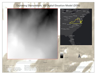
The DSM Map below depicts a DEM that I created using the LAS Dataset to Raster geoprocessing tool in ArcGIS Pro 2.4.

The Mashup map below is a concoction of efforts from this week's lab.  It shows elevation side-by-side with canopy density to infer what elevations are associated with tree density and possible soil conditions.

More details of this week's lab can be viewed on a new Esri story map I've been experimenting with this week. It is a work-in-progress story of this week's lab.  It is subject to good and bad decisions as I learn this new way to communicate location.

In Closing

I learned a lot of interesting information about LiDAR and how it is used in various industries like Forestry and Local Government.

GIS-5100 Module 1: Least Cost Path & Corridor Analysis

Overview

Week two of module 1 consisted of two main scenarios, which continued to reinforce the concept of Suitability and Least-Cost Analysis and topics such as Least Cost Path, plus Corridor Analysis.  In scenario 3, I assumed a role as a GIS Analyst working for an oil company planning to construct a pipeline outside of Medford, Oregon.  I'm tasked with performing three analyses that build off each other.  I'm told that each analysis should consider slope, river crossing, and river proximity.  I'm provided all the datasets so that I can perform the following analysis: slope, add cost for crossing rivers, add cost for proximity to rivers, which results in raster outputs of least-cost analysis.  Then I'm to input these least-cost outputs into a workflow involving Corridor Analysis, which takes into account the accumulation of all the possible paths between a source and destination point feature.  Below is the final corridor I managed to create.

Scenario 4

Next came scenario 4, which is the topic of this blog.  The goal is to repeat scenario 3.  But the scenario is a little different.  Now I'm a Park Ranger in the Coronado National Forest asked to model the potential movement of black bears between two protected areas that results in a corridor like performed in scenario 3.  Again, I first create a simple plan to document the basics statements such as Problem, Goal, Objectives, and planned deliverables.  Then I started preparing the data to create a suitability raster and cost surface raster.  Below is what my model looks like.

But now the source and destination are polygons instead of points and the criteria are slightly different. Below is an image depicting the cost surface raster with the source (Coronado1) and destination (Coronado2) areas.

What followed next was the creation of the least cost raster using the Cost Distance and Cost Path tools and the input of the previously created cost surface raster, source feature (Coronado1) and destination feature (Coronado2).  The extended workflow now looks like the image shown below.

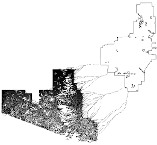
The results of the first Least-Cost Raster shown above between source and destination originally shocked me when I saw all the possible paths created by the model (see image below).

Then I added another Least-Cost Analysis to the above model to consider paths traveling in the opposite direction, destination area (Coronado2) to the source area (Coronado1).

Lastly, running the Corridor Tool was now possible by inputting the two previous Least-Cost Rasters.  Below is the final layout map created with the output of the Corridor tool.

Summary

I've tried to capture the essence of Scenario 4 Lab, which is Suitability Analysis in action.  Suitability Analysis ranks and scores locations/sites based on a few or several weighted criteria.  The number of criteria depends on the intended goal.  The suitability of a candidate location can be ranked based on data variables, site attributes, or proximity to point features.  Working out the details of important criteria with Stakeholders and subject matter experts is vital to configuring and assigning weights to determine scores for each of the potential site locations.

A few high-level assumptions worth mentioning about Suitability Analysis are:

• The Spatial Analyst extension is required to experiment with processes, procedures, and algorithms of Esri's Suitability Analysis workflow.
• Some level of comfort is helpful with Model Builder and experimenting with geoprocessing tools (about 190 now and growing).
• Map Algebra can be tricky and requires some experimentation.
• Working with rasters and doing math with them might be a new concept, it might require additional effort experimenting with them and the Raster Calculator.

Closing

Although I did not mention the creation of a plan prior to getting started, I created a template so I could quickly document the basic gist of what I'm trying to do.  I can't count the number of times I had to refer to it to reestablish my bearing by reminding myself of the goal.  I often found myself in the weeds working through the lab and venturing down rabbit holes in the quest for understanding.  Having a simple plan-do-act document is my escape hatch out of these fact-finding internet expeditions.

ArcGIS-Pro 2.4 and the Spatial Analyst Extension to model potential corridor movement for black bears between two areas of the Coronado National Forest (Santa Cruz) in Tuscon, Arizona

I'm glad to have gotten my feet wet with Suitability Analysis.  I'm planning new adventures using this technology and hope to apply it with scenarios of my own in the near future.

GIS-5100 Module 1: Understanding Suitability Analysis & Getting to know the Weighted Overlay Tool

Week one consisted of two main scenarios, which introduced me to the concept of Suitability and Least-Cost Analysis and topics such as Boolean Suitability in both Vector and Raster, rating locations in Raster, Least Cost Path, and Corridor Analysis, and many more topics related to GIS-focused approaches to Suitability Analysis.  This blog is specific to scenario 2, which put me in a position as a GIS Analyst for a property developer.  The supporting lab was quite involved with approximately 15 defined deliverables (30 deliverable for the entire Module).  I really liked learning about the various types of GIS-based processes and means of creating a workflow to model a real-world system to meet the needs of a stakeholder, Land Developer Firm. ( hmmm, sounds like project management terminology).

What followed next before cracking open ArcGIS-Pro was the creation of basic project management artifacts.  We did not formally define a scope statement, requirements document, Charter, or project management plan (PMP), but it sure felt like it when we stated a problem, goal, objectives, processes, and deliverables such as services and map products.  It's so vital to have a well-defined plan.  See a portion of the example project plan I created below.

Problem: Where are suitable locations for future Site Developments within the boundary of Land Tract?
Goal: Create a suitability model to identify the best locations for future planned urban development.
Objectives: Various items here defining the input requirements to model the desired outcomes
Workflow: See image below as an example of the partial workflow of preparing the geographic data by geoprocessing tools to support further types of analysis responsible to reach and meet the desired outcomes of stakeholders.

Analysis:
The map below is the result of modeling a system using an Esri Weighted Overlay approach of suitability analysis, which involved the use of ArcGIS Pro 2.4.0.  I definitely had a full plate this week with getting through the Lecture material, four different lab scenarios, thirty Lab deliverables, and learning how to use the Weight Overlay Tool, but it was well worth the effort and learning pains!
What's really nice about the Weighted Overlay Tools is that by adding or subtracting layers in conjunction with setting an influence/importance level to each layer, the model can generate a totally different outcome for Stakeholders to consider and make better strategic business decisions.

This week Learned Outcomes:
▪ Perform suitability analysis using both vector and raster analysis tools
▪ Prepare data for use in suitability workflows
▪ Compare different approaches to suitability analysis, including Boolean and Weighted scoring
▪ Compare vector and raster tools to complete specific steps in the suitability analysis
▪ Adjust specific parameters employed in suitability analysis, such as scoring and weighting
▪ Perform least-cost path and corridor analysis using cost surfaces
▪ Prepare elevation, land cover, and other data for use in the least-cost path and corridor analysis
▪ Create cost surfaces based on a variety of input data
▪ Interpret the results of the least-cost path and corridor analysis
▪ Adjust specific parameters employed in the least-cost path and corridor analysis

In Conclusion
This week involved tasks and activities in constructing an informal Project Management Plan, which defined end deliverables via a problem, purpose, and objectives as described by stakeholders and subject matter experts.  I spent quite some time using ArcGIS Pro, Model Builder, and overlaying several rasters and applying a common measurement scale and weights each according to its defined importance for best future Site development endeavors.

Oriention Blog

Hi there,

It's Summertime and this is my opening blog to an 8-week Applications in GIS course that is designed to introduce how to apply the use of GIS in the study of geohazards, natural disasters, urban planning, homeland security/law enforcement. and marketing/location decisions.  Laboratory exercises, case studies, and course projects are structured to use true-to-life datasets to solve real-world problems.

Getting started is always takes me extra effort to feel comfortable.  I'm sure I'll get bucked out of my saddle, but I'll brush off the dust and climb back on to find my seat again.

Talking about horses and saddles is a theme I used to create my first story map of the course.  I've always had an affection and appreciation for the western way of life, which again is the theme I expressed in my first web app. Here is a link to my Story Map: https://arcg.is/18990r0

Well now that I'm done with the formalities of orientation obligations, its time for the first GIS application, the examination of different approaches to suitability modeling.  Suitability modeling identifies the most suitable locations based on a set of criteria. It is one of the classical examples of GIS, and it represents a very well established technique that has been around since the early days of spatial analysis using GIS.

Well, I better head off to my reading assignments for module 1.

Until Next Time,